Blog

December 27th, 2020

Performance of Exchange Traded Funds in the Indian Market

By Achintya Tiwari, Abhrajit Sarkar and Atharva Mirajkar

In the early 1970s, the advantages of passive investing in the stock market started appearing in academic discussions. It really took off in the 1990s, when the general public began to realize that most Mutual funds were unable to beat the US Benchmark index. The high fees they charged for managing a portfolio wasn’t justified anymore. This led to the creation of a new instrument; the Exchange Traded Fund (ETF).

An ETF is a security listed on the stock exchange, that lets you invest in a host of different assets covered by an Index. For example, an ETF following the NIFTY 50 index will take cash from the public in exchange for shares of the ETF that are backed by stocks of the 50 companies covered by the index.

In the Indian context, a very popular alternative is a Mutual Fund. It allows investors to participate without having a DEMAT account and is considered less risky in the long term. Actively managed by a seasoned professional, they make sense if a fund is able to consistently generate good returns over the long term. However, the extra returns have begun to decrease and the costs associated with Mutual funds (1-2.5% of total assets invested, along with exit costs) eat away from profits.

The first ETF in India (NIFTY BeES) was created in 2001. Since then, several ETFs have sprung up on Indian exchanges and the total Assets under management have grown over 12X in the last five years, or at a Compound Annual Growth Rate (CAGR) of 65%. As of today, 88 ETFs are available for investors, there is no dearth of options. So how do we go about choosing one?

An attribution analysis generally gives a good picture of how well an investment has performed, compared to the market. Similarly, a multitude of ratios, such as the Sharpe ratio and the alpha measure, have been used to gauge the performance of mutual funds.  While these can be used to compare performances of funds that are managed actively, passively managed investments like ETFs cannot be looked at through the same lens.

An ETF is bound to follow the underlying index, the fund house does not decide which assets to invest in and which to avoid. So, the return profile is a direct reflection of the benchmark, which has been chosen by the investor. For example, there are 8 ETFs that follow the NIFTY 50 Index, which grew at a CAGR of 10.8% over the last 5 years. If any of these 8 were picked, 10.8% would have been the return expected over the same period. Since the benchmark is fixed, lower deviations from this benchmark signify a better-managed ETF.

How to compare ETFs?

Every fund house publishes a factsheet to release information about the ETF publicly. It contains details like Assets Under Management, date of inception, underlying benchmark, expense ratio etc. The most important of these factors listed here are the Tracking error and Expense ratio (ER).

To understand them better, we must first look at the Net Asset Value (NAV) and Market Price of an ETF. The market price is decided by the participants and is the amount paid when buying or selling a share of the ETF on the exchange. The NAV is the underlying value of 1 share held by the fund. In simpler terms, if all the assets held by the fund were divided by the number of shares in the market, we would get the NAV of the ETF. It is important to note that NAV is balanced with respect to the underlying index by a fund house at the end of each day. The market closing price is a result of the day’s trading activity.

Tracking error is the difference between an ETF portfolio's returns and the benchmark or index it was meant to mimic or beat. On a trading day, if the Underlying index rose by 0.5%, but the ETF rose by 0.4%, the return’s error for that day would be 0.1%. Over a long period, the standard deviation of this return’s error calculated daily gives us the Tracking Error of the ETF. A typical factsheet would represent it like this.

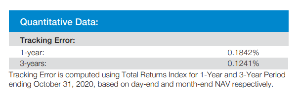
Scheme Factsheet – SBI NIFTY50

 

The existence of two numbers for the value of one share gives us two ways to calculate tracking error, one with NAV and one with the market price. Interestingly, the tracking error mentioned here is calculated using the NAV, whereas we would be gaining or losing basis points while buying/selling using the market price.

The ER is the total fees the fund house charges per year. This includes management fees and operating costs. An Expense ratio of 1% would mean that if an investment grew by 8%, the investor would only gain 7% on his investment. Most ERs of ETFs range between 0.07-1%.

Our Study

The first step was to calculate a new tracking error using the market closing price. This value would reflect the gains made by an investor better than NAV’s tracking error. We used data of the last 5 years as most ETFs weren’t trading regularly before that. The number of shares that are bought or sold (i.e., The Volume of the ETF) have really picked up only recently signifying an increasing interest and activity in ETFs. Tracking error with respect to NAV was also recalculated for this time frame.

An interesting observation was made here. The tracking error from Market data was sometimes 10X higher than that calculated from NAV. This was already enough proof that the tracking error published is not a good representation of how much an investor is going to lose or gain because of the ETF’s performance. 

To gain further insight into where this discrepancy originates, we considered the following factors:

• Expense Ratio
• The volatility of the underlying benchmark (using standard deviations of daily returns)
• Assets under management (given in the factsheets or Scheme information documents)
• Liquidity of the ETF in the market

The liquidity, or ease of entry or exit from an investment, is measured by the difference in the prices of ETFs available for purchase and sale during trading hours, i.e., the bidding price and the asking price respectively. The gap between the prices is known as the Bid-Ask spread, and access to this data for every second over the past 5 years is expensive, making it inaccessible. Trading volumes have also increased significantly over the last 5 years, so taking an average and using it as a property of the ETF would have given misleading results. Hence, a workaround to this problem is using a proxy for the spread, derived with the help of a paper referenced below.

In 1984, Richard Roll, assuming an efficient market, arrived at a formula to derive an estimated bid-ask spread using the day high, day low and closing prices. In 2017, Abdi and Ranaldo built on this study and modified the formula for less liquid and irregular stocks. The spread is given by the formula

In which c is the daily close log-price and η is the daily mid-range, that is, the average of daily high and low log-prices. This simple closed-form solution E[ ] resembles Roll’s auto-covariance measure. However, instead of the autocovariance of consecutive close-to-close price returns like in the Roll measure, this estimator relies on the covariance of close-to-mid-range returns around the same close price.

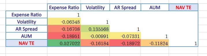
Once numerical values were obtained for all the factors mentioned above, we calculated the correlation values and have presented the results below.

 

 

 

Conclusion

From the correlation tables, we can see that NAV Tracking error correlates well with Expense ratio. This is expected, as lower costs of managing the fund mean lesser deviations from the index and vice versa. Both these figures are publicly released by the fund. For the Price derived tracking error, or real observed Tracking error, the spread has the highest correlation while the size of the funds has the lowest correlation. This means that ETFs which had a higher Price tracking error also had a higher Spread (low liquidity), and a lower fund size.

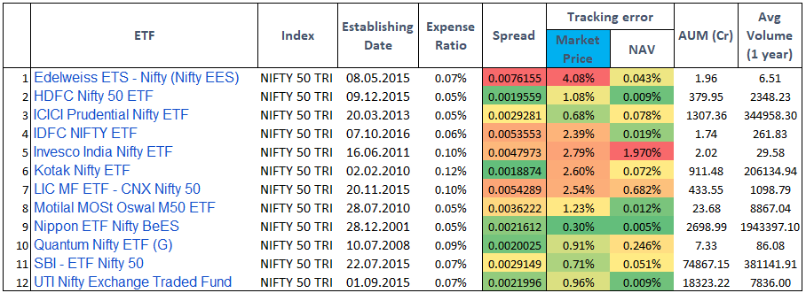
Let’s consider ETFs tracking the NIFTY 50 index to get a better understanding. The data that would be readily available are Tracking error - NAV, AUM and Expense ratio. A fund would ideally want us to make our decision based on these variables. A closer look at the table shows a different picture.

If an investor based his decisions on a low NAV tracking error, he would have encountered a low real tracking error over the last 5 years in the case of Nippon NIFTY BeES, but his expectations would have been very off in the case of Edelweiss Nifty EES. We can see that the spread even warns us about this possible issue.

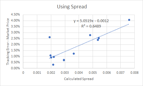
Correlation Coefficient = 0.81

R-square = 0.65

To better estimate for a lower Market price, we found that the Spread, as a measure of liquidity, was the best variable to consider. Even on conducting a linear regression we saw a good R-squared value.

If ETFs were liquid, conventional reporting by the funds could have been enough to gauge and compare ETFs. This is not the case today for most ETFs, and may not be for the near future. While investing in ETFs, we suggest a historical study of the real tracking error to seek out the ETFs which would track an index well. While this may seem easy for a couple of ETFs, it will become cumbersome while shortlisting from the universe. In this case, liquidity via a Bid-ask spread can be considered a good enough proxy for observed tracking error.

 References

1. India 2019 Mutual Fund Report http://www.citigroup.com/emeaemailresources/gra30616_2019_IndiaCountryUpdate_v9.pdf
2. Scheme Factsheet, SBI ETF NIFTY 50 https://www.sbimf.com/en-us/lists/schemefactsheets/sbi-etf nifty 50 (november-2020-433-11).pdf.pdf
3. A Simple Implicit Measure of the Effective Bid?Ask Spread in an Efficient Market - Richard roll - https://doi.org/10.1111/j.1540-6261.1984.tb03897.x
4. A Simple Estimation of Bid-Ask Spreads from Daily Close, High, and Low Prices - https://doi.org/10.1093/rfs/hhx084

Comments